Time Series Prediction with Machine Learning (Getting Started).

What is Time Series Data ?

Time series data (Time-stamped data), is a sequence of data points indexed in time order. Time-stamped is data collected at different points in time.

These data points typically consist of successive measurements made from the same source over a time interval and are used to track change over time.

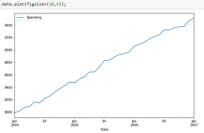
Example : Here is a Dataset which has Personal Spending's of a man from 2004–01–01 to 2007–01–01, where data is collected Periodically on the 1st day of Each Month.

What is the use of Time Series Data ?

Using Time Series data, we can find patterns in the data and this can then be used for predict/forecast the values of any given variable.

This too has its limitations, if the given variable is largely dependent on any external factors our Model will not give the best results.

However, Time Series forecasting is an important area of machine learning, because there are many prediction problems that involve time component.

There are a lot of components when doing a Time Series Analysis/Forecasting. Using the example of Personal spending dataset to do Analysis & Forecasting on it, we will look into all the components that come along with it.

1. Getting the Timeseries Data in the correct format

We will be working on the Personal Spending's dataset which has the Personal Spending’s of a man from 2004–01–01 to 2007–01–01, where data is collected Periodically on the 1st day of Each Month.

• Pass the variable which has Timestamp data to index_col and set parse_date=True , to read the data in the correct format.
• Check the frequency of our dataset (could be daily, monthly, yearly etc.)and set the index frequency accordingly.

2. EDA

• We have Monthly data, so as we have total 37 rows, the total data we have is for 3 years and 1 month (2004–01–01 to 2007–01–01).

• Plot the Data to get insights : From this Graph we cans see that there is clearly an upward Trend in the data and also some Seasonality. These 2 terms are very important in Time series analysis, so we will see what they really mean.

Important Concepts

1. Trend : The trend shows the general tendency of the data to increase or decrease during a long period of time. A trend is a smooth, general, long-term, average tendency. It is not always necessary that the increase or decrease is in the same direction throughout the given period of time. The 3 types of Trend : 1.Upward 2.Downward 3.Horizontal/Stationary
2. Seasonality : Seasonality is a characteristic of a time series in which the data experiences regular and predictable changes that recur every calendar year. Any predictable fluctuation or pattern that recurs or repeats over a one-year period is said to be seasonal
3. Stationarity : A Time Series data is said to be stationary if its statistical properties such as mean, variance remain constant over time. Most of the Time Series models work on the assumption that the data is stationary, so if our data is non-stationary we will have to convert it to stationary data. Another advantage of converting data to stationary is, the theories related to stationary data are way more mature and easy to implement.

Looking at the Plot above, we can say there is a clear upwards Trend in our data and also some seasonality. But it may not be so straightforward for all datasets. Therefore, we can use seasonal_decompose to find out if our data has Seasonality, Trend.

Seasonal Decompose

Seasonal Decompose will return 4 things :

1. Observed (Original data)
2. Trend (General trend)
3. seasonal data
4. Error/Residual (Data that cant be explained by either seasonality or seasonality)

There are 2 options for Seasonal Decompose :

1. Additive (when trend is more linear , seasonality and trend seem to be constant)
2. Multiplicative (trend is more non-linear)

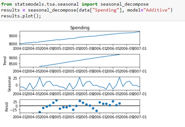
From this Image we can see that the Seasonal Decompose clearly tells us that there is some Upward Trend and some Seasonality in the Data.

3.Check For Stationarity.

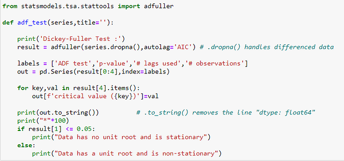
Dickey-Fuller Function : Check if data is Stationary.

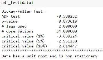
It returns a P-value, if p<0.5 : Data is Stationary , p>0.5 : Data is Not Stationary.

Function to check Stationarity using the Dickey-Fuller Test

So, After checking with this function we concluded that the data is Non-Stationary.

4. Select the Correct Model and Make the data Stationary

ARIMA : Auto Regressive Integrated Moving Average.

ARIMA is one of the best models for prediction, details here.

• To effectively use ARIMA, we need to understand the Stationarity in our data.
• IF we have determined the data is Not stationary, we will need to make it stationary to predict it.
  - One simple way to do it is Using Differencing.
• After the Data is made Stationary, we will need to choose the p, d, q parameters. (p : # of Lags in AR, d : Degree of differencing, q : Order of MA model)

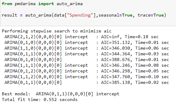
We can here use the auto_arima function to find the best values of p, d, q. we will.

auto_arima():

Automatically discover the optimal order for an ARIMA model.

The auto-ARIMA process seeks to identify the most optimal
parameters for an `ARIMA` model

So from the auto_arima(), we got the best parameters as : p=1, d=1, q=1

Output of auto_arima()

Now, we don't really need to differentiate the data to make it stationary, passing d=1 to ARIMA will differentiate it by 1 for us.

5. Build the ARIMA model, and Predict on test data.

• In ARIMA() we pass order=(p, d, q),we have passed our p, d, q which are 0, 1, 1

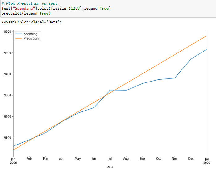
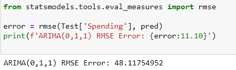
6. Plot the Predictions and evaluate the results.

This is the result we got, the output/RMSE score is decent considering we have used a simple ARIMA model and our training data is small.

Plotting the Predicted data and the Original Data.

RMSE for the Model.

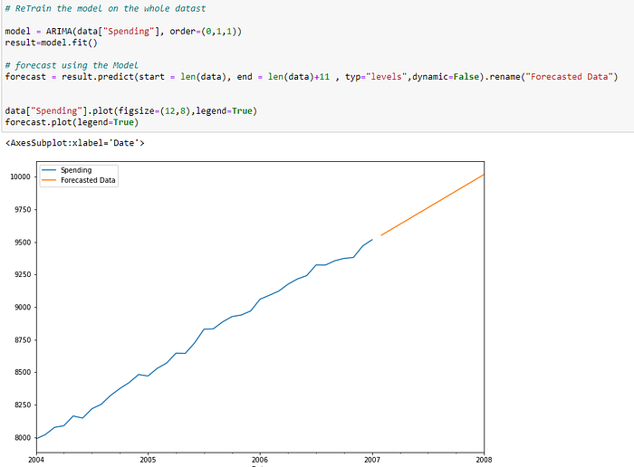
7. Forecast future data.

We will now train on the whole data (3 years) and predict for 1 year ahead.

This is it for getting started and just to get a feel of Time series prediction using a simple ARIMA model, I will some more examples where we use more complex models like SARIMA, SARIMAX and also to use multiple columns for Forecasting.

Thanks for reading :)